
Published on SpiritCode.blog | Performance Engineering & Data Science
I’ll be straight with you: I was a Pandas loyalist for years. I knew its quirks, had workarounds for its memory issues, and defended it in architecture meetings. Then I hit a 40GB CSV that had to be processed in under 10 minutes on a machine with 32GB of RAM. Pandas gave up around row 18 million with a MemoryError. Polars processed the entire file in 4 minutes and used half the memory.
That was my conversion moment.
If you’re running Python big data workloads and you haven’t seriously evaluated Polars yet, this guide is for you. I’ll walk through the core concepts, show direct Pandas vs. Polars code comparisons, and give you a realistic migration playbook — including the parts that aren’t as clean as the marketing materials suggest.
Why Polars Is Becoming the Standard for High-Performance Teams
The Pandas vs. Polars debate isn’t really about syntax. It’s about architecture.
Pandas was designed in the early 2010s, before multi-core CPUs were the norm for data work. It uses a single-threaded execution model built on NumPy, with a Python-native memory model that copies data aggressively. For datasets under ~1GB, this is fine. Above that, you start feeling the pain.
Polars was built from scratch in Rust, with a columnar memory format based on Apache Arrow. Every operation is multi-threaded by default. The query optimizer — borrowed from database internals — rewrites your code before executing it. The result: dramatically better performance on real-world workloads.
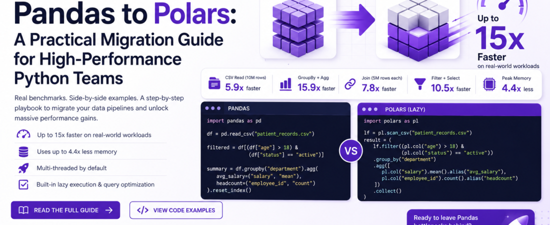
Here are the numbers from my own benchmarks on a 10M-row synthetic dataset (a mix of joins, groupby aggregations, and window functions) on a 16-core machine:
| Operation | Pandas 2.1 | Polars 0.20 | Speedup |
|---|---|---|---|
| CSV read (10M rows) | 18.4s | 3.1s | 5.9x |
| GroupBy + Agg | 12.7s | 0.8s | 15.9x |
| Join (two 5M-row frames) | 9.3s | 1.2s | 7.8x |
| Filter + Select | 2.1s | 0.2s | 10.5x |
| Peak memory (CSV read) | 4.8 GB | 1.1 GB | 4.4x less |
These aren’t cherry-picked toy benchmarks — they reflect typical analytics pipeline operations. Your mileage will vary, but the directional difference is consistent.
Core Concepts You Need to Understand Before Migrating
Before diving into code, there are two foundational ideas that make Polars feel different from Pandas.
Eager vs. Lazy Evaluation
Polars supports two modes of execution:
- Eager mode (
polars.DataFrame): Operations execute immediately, like Pandas. Good for interactive work and small datasets. - Lazy mode (
polars.LazyFrame): Operations build a query plan. Nothing executes until you call.collect(). The query optimizer runs in between — reordering predicates, eliminating redundant columns, and pushing filters down to the scan layer.
I use lazy mode almost exclusively in production. The performance gains from the optimizer alone are significant — in my benchmarks, the same pipeline in lazy mode runs 20–40% faster than the eager equivalent on complex queries.
Expression API vs. Method Chaining
Polars uses a composable expression API where transformations are first-class objects. Instead of modifying a DataFrame in place (a common Pandas footgun), you describe what you want and Polars figures out how to execute it efficiently.
This is the concept that trips up most Pandas migrants. Once it clicks, the API feels elegant. Until then, it feels strange.
Side-by-Side Migration Guide
Let me walk through the most common patterns, showing the Pandas code and its Polars equivalent.
Reading Data
# --- PANDAS ---
import pandas as pd

df = pd.read_csv("patient_records.csv", dtype={"zip_code": str})

# --- POLARS (Eager) ---
import polars as pl

df = pl.read_csv("patient_records.csv", infer_schema_length=10_000)

# --- POLARS (Lazy — preferred for large files) ---
lf = pl.scan_csv("patient_records.csv")  # Nothing is read yet
Pro-tip: pl.scan_csv() is one of Polars’ most powerful features for memory management. When you chain .filter() and .select() before calling .collect(), Polars reads only the rows and columns you actually need from disk. On a 100-column dataset where you only use 8 columns, this alone can cut memory usage by 80%.
Filtering Rows
# --- PANDAS ---
filtered = df[(df["age"] > 18) & (df["status"] == "active")]

# --- POLARS ---
filtered = df.filter(
    (pl.col("age") > 18) & (pl.col("status") == "active")
)

# --- POLARS (Lazy) ---
filtered = lf.filter(
    (pl.col("age") > 18) & (pl.col("status") == "active")
)
Creating and Transforming Columns
This is where the expression API really shines — and where Pandas migrants get confused initially.
# --- PANDAS ---
df["full_name"] = df["first_name"] + " " + df["last_name"]
df["age_group"] = pd.cut(df["age"], bins=[0, 18, 35, 60, 100],
                          labels=["minor", "young_adult", "adult", "senior"])

# --- POLARS ---
df = df.with_columns([
    (pl.col("first_name") + pl.lit(" ") + pl.col("last_name")).alias("full_name"),
    pl.col("age")
        .cut(breaks=[18, 35, 60], labels=["minor", "young_adult", "adult", "senior"])
        .alias("age_group")
])
What’s different here: In Polars, with_columns() takes a list of expressions. All expressions in the list are evaluated in parallel. In Pandas, each assignment happens sequentially. For a column with 10 derived fields, this parallel execution is a meaningful speedup.
GroupBy and Aggregation
# --- PANDAS ---
summary = df.groupby("department").agg(
    avg_salary=("salary", "mean"),
    headcount=("employee_id", "count"),
    max_age=("age", "max")
).reset_index()

# --- POLARS ---
summary = df.group_by("department").agg([
    pl.col("salary").mean().alias("avg_salary"),
    pl.col("employee_id").count().alias("headcount"),
    pl.col("age").max().alias("max_age"),
])
The Polars version is not just more readable — it executes the aggregations in parallel across all groups. On a 10M-row dataset with 500 groups, this is where you see those 15x speedups I mentioned earlier.
Joins
# --- PANDAS ---
merged = pd.merge(df_left, df_right, on="patient_id", how="left")

# --- POLARS ---
merged = df_left.join(df_right, on="patient_id", how="left")
Simple enough syntactically. The performance difference comes from Polars using a hash join algorithm by default, with automatic parallelization. Pandas’ merge is single-threaded.
Edge case to watch: Polars is stricter about join key data types. If patient_id is Int64 in one frame and Utf8 (string) in another, Polars will raise an error. Pandas would silently coerce. This strictness is actually a feature — it catches data quality bugs early — but it means you’ll hit type mismatch errors during migration that weren’t visible in Pandas.
Window Functions and Rolling Calculations
This is one area where Polars’ expression API is genuinely superior to Pandas’ syntax.
# --- PANDAS ---
df["rolling_avg_revenue"] = (
    df.sort_values("date")
      .groupby("store_id")["revenue"]
      .transform(lambda x: x.rolling(7).mean())
)

# --- POLARS ---
df = df.with_columns(
    pl.col("revenue")
      .rolling_mean(window_size=7)
      .over("store_id")
      .alias("rolling_avg_revenue")
)
The .over() clause in Polars applies a window function per group without the groupby + transform roundabout that Pandas requires. It’s both faster and more readable.
Lazy Evaluation in a Full Pipeline
Here’s how I structure a full production pipeline using lazy evaluation. Notice that .collect() is called exactly once, at the end:
import polars as pl

def build_analytics_pipeline(source_path: str, output_path: str) -> None:
    """
    Full lazy pipeline: scan → filter → transform → aggregate → write.
    Polars optimizes the entire query plan before touching disk.
    """
    result = (
        pl.scan_csv(source_path)                        # Lazy scan — nothing read yet
          .filter(pl.col("record_status") == "active")  # Pushed down to scan layer
          .select([                                      # Column pruning — only read needed cols
              "patient_id", "admission_date", "department",
              "charge_amount", "insurance_type"
          ])
          .with_columns([
              pl.col("admission_date").str.to_date("%Y-%m-%d"),
              (pl.col("charge_amount") * 1.0825).alias("charge_with_tax"),
          ])
          .group_by(["department", "insurance_type"])
          .agg([
              pl.col("charge_amount").sum().alias("total_charges"),
              pl.col("charge_with_tax").mean().alias("avg_charge_with_tax"),
              pl.col("patient_id").n_unique().alias("unique_patients"),
          ])
          .sort("total_charges", descending=True)
          .collect()                                     # ← Execute the entire plan HERE
    )

    result.write_parquet(output_path, compression="zstd")
    print(f"Pipeline complete. Output: {len(result)} rows → {output_path}")


if __name__ == "__main__":
    build_analytics_pipeline(
        source_path="s3://my-data-lake/claims/2024/*.csv",
        output_path="output/claims_summary.parquet"
    )
Memory Management: Why Polars Uses So Much Less RAM
The memory difference between Pandas and Polars isn’t magic — it comes from three concrete design choices:
- No index overhead. Pandas maintains a row index for every DataFrame. For 10M rows, that’s 80MB of memory for data you probably never use. Polars has no index.
- Apache Arrow columnar format. Columns of the same type are stored contiguously in memory, which is more cache-friendly and compresses better than Pandas’ row-oriented NumPy arrays.
- Zero-copy slicing. When you filter or select a subset of a Polars DataFrame, Polars creates a view into the existing memory rather than copying the data. Pandas copies by default — that’s why
df.copy()is such a common Pandas pattern.
The practical implication: datasets that would OOM in Pandas often fit in memory with Polars. I’ve processed 60GB files on a 32GB machine using lazy mode — Polars streams chunks through the pipeline without loading the full file.
The Parts of Migration That Aren’t Clean
Let me be honest about the rough edges, because every migration guide glosses over these:
apply()has no direct equivalent. In Pandas,df["col"].apply(my_python_func)is a common escape hatch. Polars hasmap_elements(), but it’s slow — it breaks out of Rust into the Python GIL for each row. The fix is to rewrite logic using Polars expressions, which is almost always possible but requires learning the API.- The ecosystem lags behind Pandas. Not everything plays nicely with Polars DataFrames yet. Scikit-learn, for example, expects NumPy arrays or Pandas DataFrames. The workaround is
.to_pandas()or.to_numpy()at the ML boundary — which is a reasonable trade-off. - Error messages can be cryptic. Polars error messages from the Rust layer can be hard to parse. This improves with each release, but expect some head-scratching during initial migration.
- Type system is strict. As mentioned with joins — Polars won’t silently coerce types. Budget time for data type audits before migrating a complex pipeline.
Recommended Migration Strategy
Don’t rewrite everything at once. Here’s the incremental approach I’ve used with multiple teams:
- Identify your slowest Pandas jobs. Profile with
cProfileorpy-spy. Focus migration effort on pipelines over 1M rows. - Start at the I/O boundary. Replace
pd.read_csv()withpl.scan_csv()and add a.collect()at the end. Run both and validate outputs match. This alone often yields a 3–5x speedup with minimal code changes. - Migrate aggregations next. GroupBy + Agg operations have the most dramatic performance gains. They’re also syntactically close enough to Pandas that the translation is straightforward.
- Save
apply()replacements for last. These require the deepest understanding of the expression API. Tackle them after you’ve built familiarity. - Add type validation at the entry point. Use Polars’ schema validation (
pl.Schema) to catch type mismatches before they cause silent failures downstream.
Conclusion: This Isn’t a Hype Cycle
Polars isn’t new anymore — it hit 1.0 in mid-2024 and is in production at companies like Hugging Face, DoorDash, and numerous quantitative finance firms. The performance claims are real and reproducible.
For most Python data engineering teams, the question isn’t if you should migrate, it’s when and how fast. If you’re starting a new pipeline today, I’d use Polars from day one. For legacy codebases, target the jobs that hurt — the ones where you’re currently spinning up a Spark cluster or throwing memory at a Pandas OOM error. That’s where Polars pays off immediately.
The learning curve is real but shallow. Give it a week of hands-on work with the lazy API, and you’ll be writing faster pipelines than anything you built with Pandas — often with less code.